 This document describes how to get realistic stress data (axial and angular) for various 3D structures simulated in Mechastick.
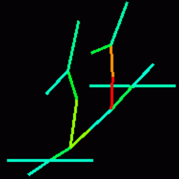
The stress for each stick should be visualized using Hue in the HSV color space – you have to develop your own (external) program that loads this kind of data and displays colored "sticks". Stress values are from zero to (theoretically) infinity.
- Download Framsticks GUI for Windows (most recent version on top)
- Run Framsticks.exe (use wine on linux or macos)
- Click the x= button on the toolbar (shows all parameters) or press ^P
- In the "Experiment definition" field, select "dump_creatures" and press "OK"
- Load (menu: File->Load) genotypes from
other.gen - Again, click the x= button on the toolbar (shows all parameters) or press ^P
- Go to "User scripts"
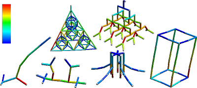
- Click the button "Make regular shapes" and close the window (ESC); several new genotypes will be added to the list
- Select any genotype on the list and drag-drop it onto the World window (it will be placed in a random location)
- The red "music player" buttons in the toolbar allow you to start ⏵︎ and stop ⏹︎ the simulation (the middle button |⏵︎ makes one simulation step). Run the simulation for just a few steps
- Now locate the
dump.txtfile in directorydata/scripts_output - This file is rewritten in each simulation step. It has all the data you need as well as explanatory comments. Ignore velocity data. Note that x and y axes constitute the horizontal plane, while z is vertical
- Place the example python script you should have available,
show_stress.py, in the same directory as thedump.txtfile, and run it - With the simulation running and the python script running, play with complex structures: add more genotypes to simulated world, use the "manipulator arm" (controlled by left mouse button + control key) to exert forces, throw balls against each other...
- Modify the python source and map linear stress values to colors linearly: 0→blue, red, yellow, >=1→white.
Additional information
- Similar visualizations: [1], [2]
- When you pressed the "Make regular shapes" button, the script
scripts/regular_shapes.scriptwas executed. You can modify itsmain()function to generate larger, sparser, or denser structures, or structures with different dimensions or with more layers - You can also build your own structure – use the simple f9 genetic format, or the more general f0 genetic format. You can start by pressing the "New" button in the "Gene pools" window and entering the genotype
/*9*/LLURRDFFUBB - Looking for more information about this simulator? check out the tutorial
- To create the
dump.txtfile in each simulation step, the function indump_creatures.incis executed – you may modify this script if needed, for example to solve the concurrent writing/reading problem by adding some end-of-file marker.
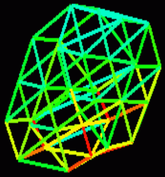
Sample output in the dump.txt file for the picture above:
# format: x1 y1 z1 x2 y2 z2 v stresslinear stressrotational
22.171 11.221 -0.279 21.885 10.935 1.079 0.0023 0.5849 0.4854
21.885 10.935 1.079 21.328 10.379 2.368 0.0062 0.5161 0.2210
21.328 10.379 2.368 20.653 9.704 3.638 0.0139 0.4463 0.0624
20.653 9.704 3.638 20.006 9.057 5.005 0.0232 0.3768 0.2747
22.154 15.213 -0.128 21.817 14.786 1.400 0.0014 0.3905 0.3626
21.817 14.786 1.400 21.236 14.204 2.892 0.0055 0.3224 0.1489
21.236 14.204 2.892 20.555 13.559 4.397 0.0120 0.2536 0.0458
20.555 13.559 4.397 19.905 12.921 5.989 0.0196 0.1845 0.1822
26.163 11.204 -0.128 25.736 10.868 1.400 0.0014 0.3905 0.3626
25.736 10.868 1.400 25.153 10.286 2.892 0.0055 0.3224 0.1489
25.153 10.286 2.892 24.508 9.606 4.397 0.0120 0.2536 0.0458
24.508 9.606 4.397 23.871 8.956 5.989 0.0196 0.1845 0.1822
26.088 15.138 0.093 25.610 14.661 1.738 0.0018 0.2390 0.2041
25.610 14.661 1.738 25.019 14.069 3.388 0.0063 0.1692 0.0673
25.019 14.069 3.388 24.388 13.439 5.084 0.0128 0.0997 0.0290
24.388 13.439 5.084 23.771 12.821 6.862 0.0195 0.0321 0.0739
22.171 11.221 -0.279 22.157 13.207 -0.062 0.0007 0.1304 0.1493
22.157 13.207 -0.062 22.154 15.213 -0.128 0.0002 0.2699 0.2824
22.171 11.221 -0.279 24.157 11.207 -0.062 0.0007 0.1304 0.1493
24.157 11.207 -0.062 26.163 11.204 -0.128 0.0002 0.2699 0.2824
22.154 15.213 -0.128 24.121 15.177 -0.009 0.0000 0.2091 0.0583
24.121 15.177 -0.009 26.088 15.138 0.093 0.0011 0.1734 0.2207
26.163 11.204 -0.128 26.126 13.172 -0.009 0.0000 0.2091 0.0583
26.126 13.172 -0.009 26.088 15.138 0.093 0.0011 0.1734 0.2207
20.006 9.057 5.005 19.951 10.992 5.460 0.0267 0.1023 0.0324
19.951 10.992 5.460 19.905 12.921 5.989 0.0245 0.0354 0.0646
20.006 9.057 5.005 21.941 9.001 5.460 0.0267 0.1023 0.0324
21.941 9.001 5.460 23.871 8.956 5.989 0.0245 0.0354 0.0646
19.905 12.921 5.989 21.841 12.867 6.389 0.0231 0.1099 0.0278
21.841 12.867 6.389 23.771 12.821 6.862 0.0227 0.0429 0.0704
23.871 8.956 5.989 23.817 10.891 6.389 0.0231 0.1099 0.0278
23.817 10.891 6.389 23.771 12.821 6.862 0.0227 0.0429 0.0704
20.006 9.057 5.005 19.410 8.461 5.153 0.0292 0.0347 0.0001
Sample visual output: