
This encoding is in many aspects similar to f1, but uses solid shapes (ellipsoids, cuboids and cylinders) and converts fS genotypes to f0s. Full sources are available in our svn repository as a part of Framsticks SDK. This description is a part of master's thesis of Jakub Sztyma supervised by Maciej Komosinski.
The fS encoding is an open-ended (it can change the structure of the phenotype), indirect, tree-like encoding designed for solid type agents. It can be used to encode both the body and the brain of agents.
1. Syntax
1.1. Creature body
A body is built like a tree. Every shape has a corresponding letter:
The shape specifier must be uppercase. If a node has only one direct child, the genes of the child begin directly after the genes of the parent. For instance, /*S*/CR represents a cuboid, which has only one child – a cylinder. If a node has several children, they need to be specified in parentheses “()” and be separated by the “,” symbol. For instance, /*S*/C(R,E) represents a cuboid, which has two children – a cylinder and an ellipsoid:
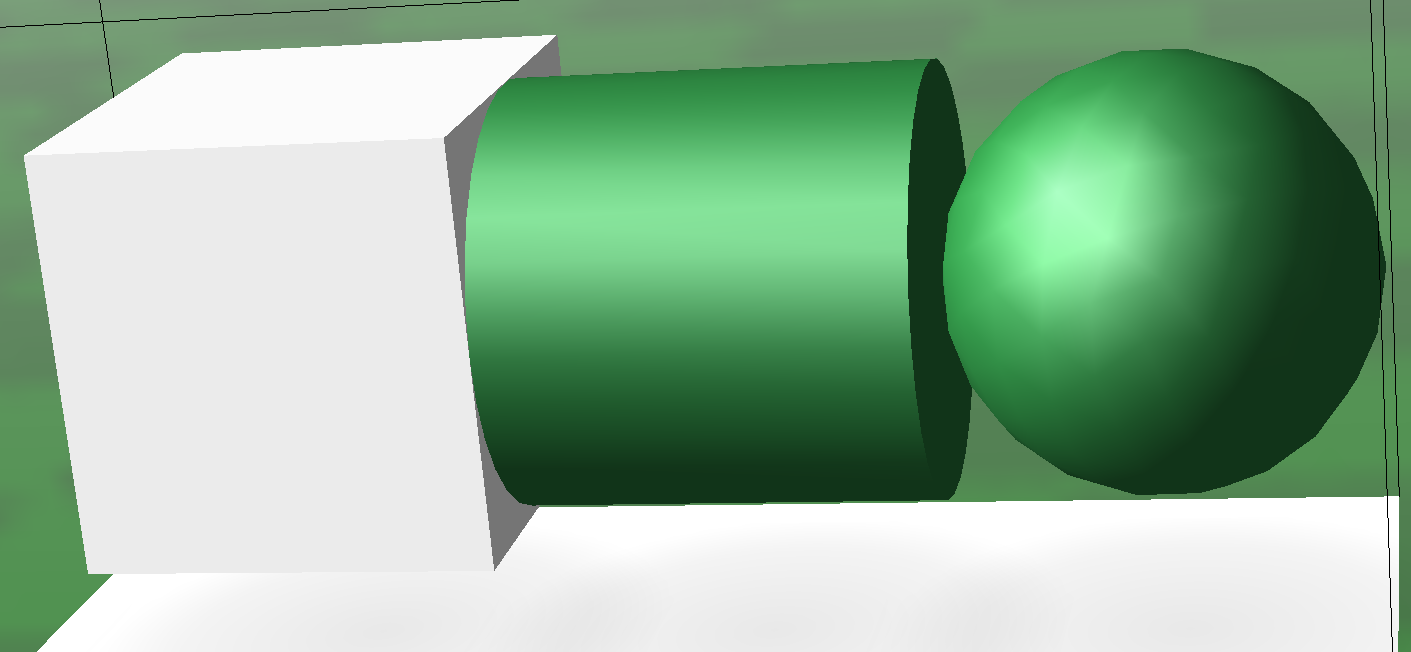 | 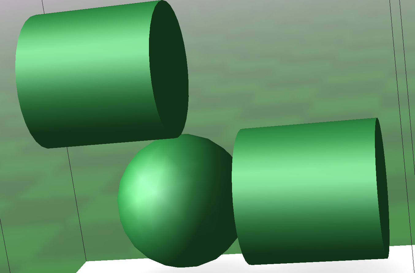 | 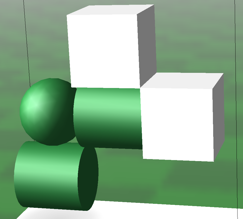 |
| /*S*/CRE | /*S*/E(R{ty=1.57},R) | /*S*/E(R{ty=-1.57},R(CC{ty=1.57}) |
1.1.1. Joints
Between the parent and each of its children, a single joint is specified. The default joint is a solid joint, which means that it can not move or bend in any axis. If there is no joint specifier between the part and its parent, it means that the default joint is used in the phenotype.
- /*S*/EE – means that the parts are connected by a fixed joint.
- /*S*/EbR – parts are connected by a hinge joint.
- /*S*/ERcC – the first and the second are connected by solid joint, the second and third by ball and socket joint.
The joint type must be lowercase.
1.1.2. Modifiers and parameters
There are two ways of modifying the properties of parts and joints.
Modifiers change the location and other properties of all parts in the entire subtree by a fixed factor. Using them can make the genotype concise. They have to be specified between the node and its parent. The available modifiers are presented below:
| Modifier letter | Affected property |
| Ss | Size of parts |
| Ii | Ingestion |
| Ff | Friction |
The uppercase modifiers increase the specified property, and lowercase modifiers decrease them. Any number of modifiers of the same type can be specified, and their effect cumulates multiplicatively. If every modifier multiplies the property by 1.1 (which is the default value but can be changed, as will be described later), the following genotypes will be translated as follows:
- /*S*/ESEE – The first part has the default size. The size (the length of each of the radiuses) of the second and the third parts are multiplied by 1.1.
- /*S*/EssEE – The size of the second and the third parts are multiplied
by
0.83 = ⋅
⋅ .
.
- /*S*/ESSSEssE – The size of the second part is multiplied by 1.33 = 1.1⋅
1.1⋅1.1. The size of the third part is multiplied by 1.1 = 1.1⋅1.1⋅1.1⋅
 ⋅
⋅ .
.
Parameters change the properties of a single node, on which they are specified. Using them enables the more precise determination of attribute values than with modifiers. They need to be specified in curly braces “{}” after the node shape specifier. If a parameter is not specified, the default value is assumed. The available parameters are listed below:
| Parameter key | Description |
| s | Size of part |
| sx | The x radius of part |
| sy | The y radius of part |
| sz | The z radius of part |
| tx | Turn on x axis |
| ty | Turn on y axis |
| tz | Turn on z axis |
| rx | The x rotation of part |
| ry | The y rotation of part |
| rz | The z rotation of part |
| f | Friction |
| i | Ingestion |
For instance, in genotype /*S*/E{f=0.3;rx=0.6;s=1.15} the specified parameters are f, rx, and s, and all other properties will get default values.
The final value of a given property derives from all modifiers specified for the node and all its parents and from the corresponding parameter. Furthermore, the value of every radius depends on the s parameter and one of sx, sy, sz parameters. For instance, the length of sx radius of the second part in genotype /*S*/SSESE{ s=1.2;sx=1.3} is equal to 2.08.
 |
1.2. Creature brain
The brain comprises of neurons and neural connections. Neurons are placed in braces “[ ]” after the node shape specifier. The following information can be supplied inside square brackets:
- Neuron type
- Properties (parameters) of the neuron
- Inputs of the neuron (if it can have inputs)
There are many types of neurons available in Framsticks. Some of them must be attached to a part, some of them – to a joint, and some may be unattached.
If multiple neurons are specified for a single node, they need to be separated by the “;” sign. Neurons are attached to the corresponding part or joint depending on the neuron type. For instance, in genotype /*S*/E[N;N]E[N] the first and the second neuron are attached to the first part, and the third neuron is attached to the second part. If a neuron has inputs, they are separated by the “,” sign.
1.3. Genotype parameters
There are several parameters that globally affect the genotype.
- Modifier factor – the factor by which every modifier multiplies the corresponding property.
- Turn with rotation – decides if the turning of a subtree during development will affect the rotation of parts in that subtree.
- Parameter mutation standard deviation – specifies the standard deviation in “change parameter” mutation.
Genotype parameters should be separated by a comma “,” and be placed before the rest of the genotype (a colon “:” is placed between genotype parameters and the genotype). Genotype parameters must be specified in a given order. For instance, in /*S*/1.3,1,0.5:E the “modifier factor” is equal to 1.3, “turn with rotation” is equal to 1 and the “parameter mutation standard deviation” is equal to 0.5. If any of the genotype parameters are omitted, the default value is assumed. In genotype /*S*/,,:E all genotype parameters are omitted, so all of them have the default value:
| Parameter | Default value |
| Modifier factor | 1.1 |
| Turn with rotation | 0 |
| Parameter mutation standard deviation | 0.4 |
2. Genetic operators
2.1. Mutation
The following mutation types have been implemented in fS:
- Add part
- Change part shape
- Remove part
- Change joint
- Add parameter
- Change parameter value
- Remove parameter
- Modify modifier
- Add neuron
- Remove neuron
- Add neuron input
- Change neuron input weight
- Remove neuron input
- Modify neuron parameters
Most of the mutations are simple – they randomly choose a place in the genotype where the specified operation can be performed, and then perform it. However, several limitations have been designed to improve the performance in evolution.
A node that has children can’t be removed in mutation. Thereby, it is impossible to remove a whole subtree in a single mutation. Neuron inputs can be created only for neuron types that accept inputs. Changing modifiers and parameters is restricted by the allowed size and shape of body parts. A mutation that violates any of the limitations is considered invalid.
It has been assumed that the volume of the part is a more important property (because it directly affects mass due to constant density) than any of the radiuses. Consequently, the “change part shape” mutation has been implemented to preserve the volume of the part and observe its allowed range. To achieve that, the radiuses of the part are recalculated accordingly.
2.2. Crossover
Crossover is implemented as an exchange of subtrees between two genotypes. To follow the postulate that “the children should not differ from parents more than parents differ from one another”, two subtrees with similar sizes (the number of nodes) are searched for. As a result, children have a similar size to their parents. Neurons that were attached to parts or joints stay attached to them. After that, new neuron connections are created in the place of neuron connections that were broken by swapping the subtrees.
3. Part size and shape control
For simulating solid shapes, Framsticks uses the ODE (Open Dynamics Engine) simulator, which currently does not support simple cylinders and ellipsoids with cross-sections other than circular. Thus, in fS, a mechanism has been implemented that controls the cross-sections of parts. The mechanism can be easily switched on and off, but for simulation in ODE it should always be active; otherwise the simulation engine will simulate solids with circular cross-section even though the phenotype will be built without such assumption.
Furthermore, in the world of solid shapes of the same density where the mass depends directly only the volume, it would be undesirable to simulate very small and very big parts within a single structure, because this would cause huge disproportion in masses and small masses would be insignificant. Thus, the size and shape of the parts are validated as follows. If any of the part radiuses is higher than allowed, the part is larger than allowed or the section of cylinder or ellipsoid is not circular, the genotype is considered invalid. All mutations are aware of these constraints and they produce genotypes with allowed size and shape.
4. Volume control
It is known that when the cuboid, ellipsoid, and cylinder all have the same radiuses, the volume of every one of them will be different (for simplicity, the half of the cuboid’s side or cylinder’s height is called a radius in this work). That means that after mutating the kind of shape of the part, the volume would change significantly. That is undesired because the phenotype would change a lot (the mass of parts would change), while we want the changes caused by a mutation to be small. To handle this problem, the volume is invariable in the “change part shape” mutation, and the radiuses are modified as appropriate to preserve volume.
Appendix. Computing the distance between parts. Internals and technical details not required to understand the genetic encoding.
A precise, analytical computation of distances between the three basic solid shapes that have any scale and any orientation in space is in general a difficult task. To calculate the approximate distance between the parent and its child, a simple algorithm has been used employing the existing functionality available in Framsticks SDK geometry module.
First, a certain number of surface points (determined by relative density
parameter) is found for one of the parts. The points are used in isCollision
method, which checks if any of the points is localized inside the second part.
The second part is initially placed at some distance from the points (in the
direction determined by the tx, ty, tz parameters). If there is a collision
between the part and the points, this distance is increased, otherwise it is
decreased. The binary search is used in order to make this procedure efficient and
convergent. The initial lower bound is the minimal theoretical distance (the sum of
minimal radiuses) and the upper bound is the maximal theoretical distance
( ⋅ sum_of _maximal_radiuses). When the distance between the lower and the
upper bound is lower than the specified tolerance, the procedure ends and returns the
current distance.
⋅ sum_of _maximal_radiuses). When the distance between the lower and the
upper bound is lower than the specified tolerance, the procedure ends and returns the
current distance.
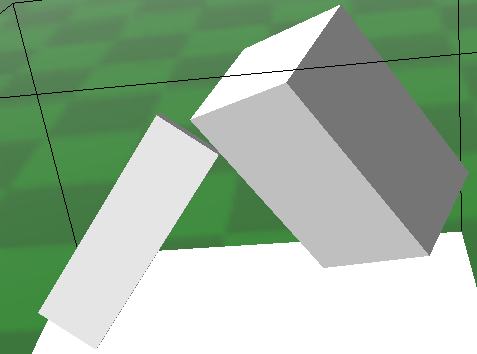
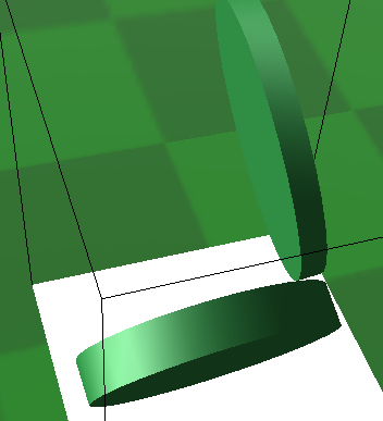
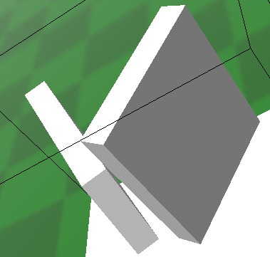
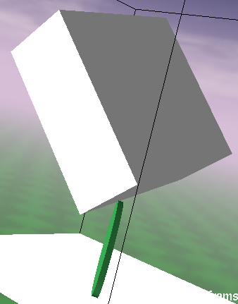
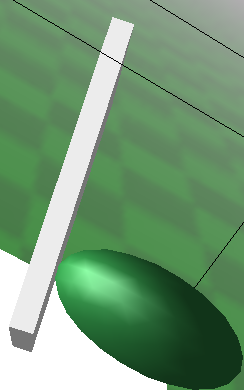
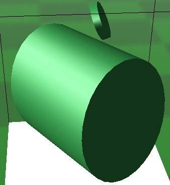
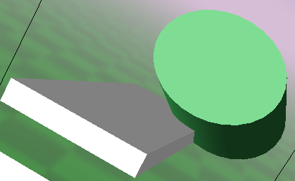
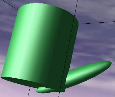
The above-described method can be parametrized. When the tolerance is low and the relative density is high, the algorithm provides very precise results. In most cases, the parts seem to be adjacent. However, with such parameter values, the computation time is high. It is important to choose such values of parameters that will provide satisfactory results while keeping the computation time low. Fig. 1.2 shows several phenotypes that were translated with parameter values that ensure high precision.
 |  |
| (a) | (b) |
 |  |
| (c) | (d) |
 | 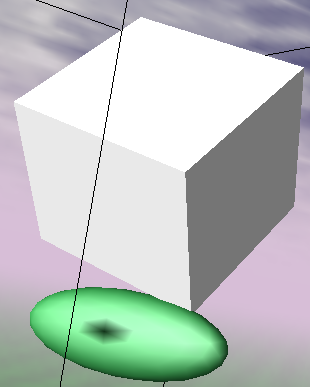 |
| (e) | (f) |
To investigate how the values of parameters affect the precision of calculated distance and the computation time, the following experiment has been conducted. 1,000 genotypes, consisting of two parts with randomly chosen values of size and rotation parameters, have been prepared. For every genotype, the reference distance (computed by the algorithm with very high density and low tolerance) and the time of conversion without computing the distance has been estimated. Then, for a range of parameter values, the following values have been calculated:
- The normalized difference between the reference results and the obtained
results; relative_difference =
 .
.
- The relative time of computation; relative_time =
 .
.
The results have been averaged for all prepared genotypes. To visualize how the value of normalized difference affects the phenotype, the following examples are presented Fig. 1.3.
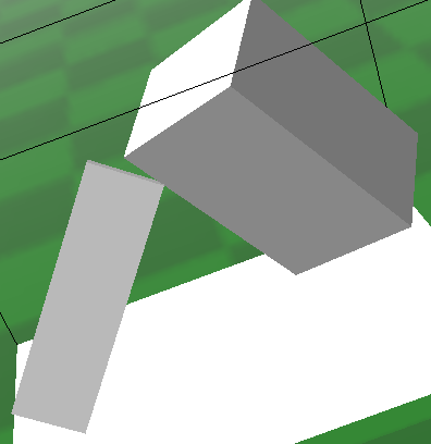 |  |
| (a) relative_difference = 0.001 | (b) relative_difference = 0.004 |
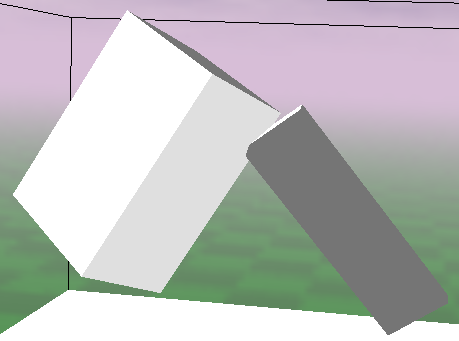 |  |
| (c) relative_difference = 0.014 | (d) relative_difference = 0.04 |
 |  |
| (e) relative_difference = 0.18 | (f) relative_difference = 0.75 |
When the relative difference is less than or equal to 0.002, the error is indiscernible. In the range between 0.002 and 0.02, the error is visible but it seems to be insignificant. For the value between 0.02 and 0.1, the error starts to be significant. For values higher than 0.1, the error is very significant – sometimes it is difficult to discover the intention (as expressed by the genotype) based on how the phenotype looks.
To make the algorithm work reasonably, the relative difference should be below 0.02. On the other hand, in most cases we want the conversion to be relatively fast, so we don’t want the algorithm to work much longer than the rest of the conversion logic. From the range of examined parameter values, we will try to choose such values that the relative difference is lower than 0.02, and the relative time is lower than 2. Figs. 1.4, 1.5, 1.6 and 1.7 plot the relative difference and the relative time of computation for different values of parameters.


When the relative density is greater than 10, the relative time is more than 3, but for values lower than 10, the relative difference is higher than necessary. Therefore, the best value of relative density seems to be around 10. The tolerance parameter seems to be less significant for precision, but for values less than 0.05 the computation time quickly increases. It seems that a value of around 0.1 would be suitable. Based on these considerations, the selected values of parameters in the fS encoding are tolerance = 0.1 and relative_density = 10.

